🔬 การวิเคราะห์ภาพ X-ray ด้วย CNN และ LLM
🎯 บทนำ: ทำไมต้องใช้ AI ในการวิเคราะห์ภาพทางการแพทย์
🏥 ความท้าทายในวงการแพทย์
การวินิจฉัยโรคจากภาพ X-ray ต้องอาศัยความเชี่ยวชาญสูง แต่ในหลายพื้นที่ยังขาดแคลนรังสีแพทย์ AI จึงเข้ามาช่วยเป็น "ผู้ช่วยแพทย์" ในการคัดกรองเบื้องต้นได้อย่างรวดเร็วและแม่นยำ
📊 ข้อมูลโปรเจกต์
- ภาพ X-ray ทั้งหมด: 5,856 ภาพ
- ปอดปกติ: 1,583 ภาพ
- ปอดอักเสบ: 4,273 ภาพ
🎯 เป้าหมาย
- คัดกรองผู้ป่วยเบื้องต้น
- ลดภาระงานแพทย์
- เพิ่มความเร็วในการวินิจฉัย
🧠 พื้นฐาน Convolutional Neural Network (CNN)
CNN คืออะไร?
Convolutional Neural Network (CNN) เป็น Deep Learning สถาปัตยกรรมที่ออกแบบมาเพื่อประมวลผลข้อมูลแบบ Grid (เช่น รูปภาพ) โดยเลียนแบบการทำงานของ Visual Cortex ในสมองมนุษย์
องค์ประกอบหลักของ CNN
สถาปัตยกรรม CNN ในโปรเจกต์นี้
ภาพ X-ray ขนาด 350×350×1 (Grayscale)
Output: 348×348×32
หาขอบและรูปร่างพื้นฐาน
Output: 174×174×32
ลดขนาดภาพครึ่งหนึ่ง
Output: 86×86×32
หารายละเอียดเพิ่มเติม
Output: 42×42×64
หารูปแบบที่ซับซ้อน
Output: 20×20×64
หาลักษณะเฉพาะของโรค
Output: 20×20×128
รวบรวมข้อมูลทั้งหมด (last_conv_layer)
Output: 51,200 neurons
แปลงเป็นข้อมูลเส้นตรง
วิเคราะห์และสกัด features
Output: ความน่าจะเป็น 0-1
(0=Normal, 1=Opacity/Pneumonia)
การทำงานของแต่ละ Layer
🔍 Convolution Layer
ทำหน้าที่คล้ายการใช้แว่นขยายสแกนทีละส่วนของภาพ เพื่อหาลักษณะสำคัญ (Features) เช่น:
- ขอบของวัตถุ (Edges)
- มุมและรูปร่าง (Corners and Shapes)
- พื้นผิว (Textures)
- รูปแบบที่ซับซ้อน (Complex Patterns)
Conv2D(32, kernel_size=(3, 3), activation='relu')
# 32 = จำนวน filters (ตัวกรอง)
# (3, 3) = ขนาดของ kernel
# relu = activation function
📉 Pooling Layer
ลดขนาดข้อมูลแต่เก็บข้อมูลสำคัญไว้ ช่วยให้:
- ลดจำนวน parameters ที่ต้องเรียนรู้
- ป้องกัน overfitting
- เพิ่มความเร็วในการประมวลผล
MaxPooling2D(pool_size=(2, 2))
# เลือกค่าสูงสุดจากทุกๆ 2×2 พิกเซล
# ลดขนาดภาพลงครึ่งหนึ่ง
🧮 Dense Layer
รวบรวมข้อมูลทั้งหมดเพื่อตัดสินใจ:
- รับข้อมูลจาก Flatten layer
- วิเคราะห์ความสัมพันธ์ของ features
- ให้ผลลัพธ์สุดท้าย
Dense(128, activation='relu')  # Hidden layer
Dense(64, activation='relu')   # Hidden layer
Dense(1, activation='sigmoid') # Output layer
🏋️ กระบวนการ Training Model
ขั้นตอนการ Train CNN Model
1. การเตรียมข้อมูล (Data Preparation)
# แบ่งข้อมูลเป็น 3 ส่วน
train_dir = 'train'      # 70% สำหรับ training (4,192 ภาพ)
val_dir = 'val'          # 15% สำหรับ validation (1,040 ภาพ)
test_dir = 'test'        # 15% สำหรับ testing (624 ภาพ)

# Data Augmentation - สร้างภาพเพิ่มจากภาพเดิม
train_datagen = ImageDataGenerator(
    rescale=1./255,           # ปรับค่าพิกเซล 0-255 → 0-1
    shear_range=0.2,          # บิดภาพ
    zoom_range=0.2,           # ซูมเข้า-ออก
    horizontal_flip=True      # พลิกภาพซ้าย-ขวา
)
เป็นเทคนิคการสร้างภาพใหม่จากภาพเดิม เพื่อเพิ่มความหลากหลายของข้อมูล ช่วยให้โมเดลเรียนรู้ได้ดีขึ้นและป้องกัน overfitting
2. การจัดการ Class Imbalance
# คำนวณ class weights เพื่อแก้ปัญหา imbalanced data
# Normal: 1,082 ภาพ (weight = 1.94)
# Pneumonia: 3,110 ภาพ (weight = 0.67)

weights = compute_class_weight(
    class_weight='balanced',
    classes=np.unique(train_generator.classes),
    y=train_generator.classes
)
เมื่อข้อมูลไม่สมดุล (ภาพปอดอักเสบมากกว่าปกติ 3 เท่า) โมเดลอาจเรียนรู้แบบลำเอียง จึงต้องใช้ class weights ปรับสมดุล
3. การ Compile และ Train Model
# Compile model
model.compile(
    optimizer='adam',              # Algorithm สำหรับ optimize
    loss='binary_crossentropy',    # Loss function สำหรับ binary classification
    metrics=['accuracy']            # ติดตามความแม่นยำ
)

# Train model
epochs = 30
history = model.fit(
    train_generator,
    callbacks=[learning_rate_reduction],
    steps_per_epoch=train_generator.samples // batch_size,
    epochs=epochs,                      # จำนวนรอบการเรียนรู้ 30 รอบ
    validation_data=validation_generator,
    validation_steps=validation_generator.samples // batch_size,
    class_weight=cw                      # ใช้ class weights
)
4. Learning Rate Scheduling
learning_rate_reduction = ReduceLROnPlateau(
    monitor='val_loss',    # ติดตาม validation loss
    patience=2,            # รอ 2 epochs ถ้าไม่ดีขึ้น
    factor=0.1,           # ลด learning rate 10 เท่า
    min_lr=0.000001       # ค่าต่ำสุดของ learning rate
)
• Epoch 1: Accuracy = 73.91%, Val Accuracy = 91.99%
• Epoch 10: Accuracy = 94.35%, Val Accuracy = 95.31%
• Epoch 30: Accuracy = 94.87%, Val Accuracy = 95.12%
• Learning rate ถูกปรับลดอัตโนมัติเมื่อ validation loss ไม่ดีขึ้น
📊 การประเมินผล Model
Confusion Matrix
Confusion Matrix แสดงผลการทำนายเทียบกับความจริง ช่วยให้เข้าใจว่าโมเดลผิดพลาดอย่างไร
| Confusion Matrix | Predicted | ||
|---|---|---|---|
| Normal | Pneumonia | ||
| Actual | Normal | 204 (TN) | 30 (FP) |
| Pneumonia | 23 (FN) | 367 (TP) | |
ความแม่นยำรวม
ความแม่นยำเมื่อทายว่าป่วย
จับผู้ป่วยจริงได้
ค่าเฉลี่ย Precision-Recall
📈 ตัวชี้วัดสำคัญ (Metrics)
= (TP + TN) / ทั้งหมด = (367 + 204) / 624 = 91.51%
บอกว่าโมเดลทายถูกกี่เปอร์เซ็นต์
= TP / (TP + FP) = 367 / (367 + 30) = 92.44%
เมื่อโมเดลบอกว่าเป็นปอดอักเสบ มีโอกาสถูกเท่าไหร่
= TP / (TP + FN) = 367 / (367 + 23) = 94.10%
จากผู้ป่วยจริงทั้งหมด โมเดลจับได้กี่เปอร์เซ็นต์
= 2 × (Precision × Recall) / (Precision + Recall) = 93.27%
ค่าเฉลี่ยฮาร์โมนิกระหว่าง Precision และ Recall
ROC Curve และ AUC
AUC = 0.9564 (ยิ่งใกล้ 1 ยิ่งดี, 0.5 = ทายมั่ว)
# คำนวณ ROC และ AUC
fpr, tpr, threshold = roc_curve(test_generator.classes, y_score)
roc_auc = auc(fpr, tpr)  # AUC = 0.9564
🤖 หลักการทำงานของ Large Language Model (LLM)
LLM คืออะไร?
Large Language Model (LLM) เป็นโมเดล AI ขนาดใหญ่ที่ถูกฝึกด้วยข้อมูลข้อความมหาศาล สามารถเข้าใจและสร้างข้อความที่มีความหมาย รวมถึงวิเคราะห์รูปภาพได้ (Multimodal LLM)
MedGemma - LLM สำหรับการแพทย์
🏥 MedGemma-4B-IT
- ขนาด 4 พันล้าน parameters
- ความสามารถ วิเคราะห์ภาพทางการแพทย์และให้คำอธิบาย
- การฝึก ใช้ข้อมูลทางการแพทย์เฉพาะทาง
- Multimodal รับทั้งข้อความและรูปภาพ
หลักการทำงานของ LLM
แปลงข้อความ/ภาพเป็น tokens
แปลง tokens เป็นเวกเตอร์ตัวเลข
ประมวลผลด้วย Attention Mechanism
สร้างคำตอบทีละ token
Attention Mechanism
# การใช้ MedGemma วิเคราะห์ภาพ X-ray
pipe = pipeline(
    "image-text-to-text",
    model="google/medgemma-4b-it",
    torch_dtype=torch.bfloat16,
    device="cuda"
)

messages = [{
    "role": "user",
    "content": [
        {"type": "text", "text": "Describe this X-ray"},
        {"type": "image", "image": xray_image}
    ]
}]

# โมเดลจะวิเคราะห์และให้คำอธิบายทางการแพทย์
💻 อธิบาย Code ใน Pneumonia.ipynb
📦 1. Import Libraries และเตรียมข้อมูล
import tensorflow as tf
from tensorflow.keras.preprocessing.image import ImageDataGenerator
import matplotlib.pyplot as plt
from PIL import Image
import numpy as np

# Download dataset จาก Kaggle
import kagglehub
path = kagglehub.dataset_download("pcbreviglieri/pneumonia-xray-images")
🖼️ 2. การโหลดและแสดงภาพตัวอย่าง
# กำหนด path ของแต่ละ class
normal_path = os.path.join(train_path, 'normal')
opacity_path = os.path.join(train_path, 'opacity')

# แสดงภาพตัวอย่าง
plt.figure(figsize=(10, 5))
normal_img = Image.open(normal_img_path)
plt.imshow(normal_img, cmap='gray')
plt.title('Normal')
plt.show()
🔄 3. Data Generator และ Augmentation
# สร้าง ImageDataGenerator สำหรับ training
train_datagen = ImageDataGenerator(
    rescale=1./255,        # Normalize pixels to [0,1]
    shear_range=0.2,       # Random shearing
    zoom_range=0.2,        # Random zoom
    horizontal_flip=True   # Random horizontal flip
)

# Load images from directories
train_generator = train_datagen.flow_from_directory(
    train_dir,
    target_size=(350, 350),  # Resize all images
    batch_size=32,           # Process 32 images at a time
    class_mode='binary',     # Binary classification
    color_mode='grayscale'   # Use grayscale images
)
• ค่าพิกเซลเดิม: 0-255
• หลัง normalize: 0-1
• ช่วยให้โมเดลเรียนรู้ได้เร็วและเสถียรกว่า
🏗️ 4. สร้างโครงสร้าง CNN Model
# สร้างโมเดลด้วย Functional API
# Input
inputs = tf.keras.Input(shape=(350, 350, 1))

# Feature Extraction
x = tf.keras.layers.Conv2D(32, (3, 3), activation='relu')(inputs)
x = tf.keras.layers.MaxPooling2D((2, 2))(x)

x = tf.keras.layers.Conv2D(32, (3, 3), activation='relu')(x)
x = tf.keras.layers.MaxPooling2D((2, 2))(x)

x = tf.keras.layers.Conv2D(64, (3, 3), activation='relu')(x)
x = tf.keras.layers.MaxPooling2D((2, 2))(x)

x = tf.keras.layers.Conv2D(64, (3, 3), activation='relu')(x)
x = tf.keras.layers.MaxPooling2D((2, 2))(x)

x = tf.keras.layers.Conv2D(128, (3, 3), activation='relu', padding='same', name='last_conv_layer')(x)

# Image Classification
x = tf.keras.layers.Flatten()(x)
x = tf.keras.layers.Dense(128, activation='relu')(x)
x = tf.keras.layers.Dense(64, activation='relu')(x)
outputs = tf.keras.layers.Dense(1, activation='sigmoid')(x)

# Model
model = tf.keras.Model(inputs=inputs, outputs=outputs)
⚖️ 5. จัดการ Class Imbalance
# นับจำนวนภาพในแต่ละ class
from collections import Counter
Counter(train_generator.classes)
# Output: {0: 1082, 1: 3110}  # Normal:Opacity ratio

# คำนวณ class weights
from sklearn.utils.class_weight import compute_class_weight
weights = compute_class_weight(
    'balanced',
    np.unique(train_generator.classes),
    train_generator.classes
)
# weights = [1.937, 0.674]  # Give more weight to minority class
🎯 6. Training และ Callbacks
# Learning rate scheduler
learning_rate_reduction = ReduceLROnPlateau(
    monitor='val_loss',
    patience=2,         # Wait 2 epochs
    factor=0.1,        # Reduce LR by factor of 10
    verbose=1,
    min_lr=0.000001
)

# Train the model
history = model.fit(
    train_generator,
    epochs=10,
    validation_data=validation_generator,
    callbacks=[learning_rate_reduction],
    class_weight=dict(zip(np.unique(train_generator.classes), weights))
)
📊 7. การประเมินผลและ Visualization
# Evaluate on test set
loss, accuracy = model.evaluate(test_generator, steps=test_generator.samples // batch_size)
print(f"Test Loss: {loss:.4f}")
print(f"Test Accuracy: {accuracy:.4f}")

# Generate predictions
predicted_classes = (model.predict(test_generator, verbose=1) > 0.5).astype("int32")[:,0]

# Create confusion matrix
from sklearn.metrics import confusion_matrix, classification_report
cm = confusion_matrix(test_generator.classes, predicted_classes)

# Generate classification report
report = classification_report(
    test_generator.classes,
    predicted_classes,
    target_names=['normal', 'opacity'],
    digits=4
)
📈 8. ROC Curve และ AUC
# Calculate ROC curve
from sklearn.metrics import roc_curve, auc

y_score = model.predict(test_generator)
y_score = y_score[:,0]
fpr, tpr, threshold = roc_curve(test_generator.classes, y_score)
roc_auc = auc(fpr, tpr)

# Plot ROC curve
import plotly.express as px
roc_df = pd.DataFrame({
    'False Positive Rate': fpr,
    'True Positive Rate': tpr,
    'Threshold': threshold
})

fig = px.area(
    roc_df,
    x='False Positive Rate',
    y='True Positive Rate',
    title=f'ROC Curve (AUC={roc_auc:.4f})'
)
💾 9. บันทึกโมเดล
# Save the trained model
model.save('pneumonia_detection_model.keras')

print("Model saved successfully as 'pneumonia_detection_model.keras'")
🔍 10. GradCAM Visualization
📖 สำหรับคำอธิบายหลักการโดยละเอียด ดูได้ที่หัวข้อ GradCAM: Explainable AI
# ติดตั้ง tf-keras-vis
!pip install tf-keras-vis

# หา last convolutional layer
for layer in reversed(model.layers):
    if isinstance(layer, tf.keras.layers.Conv2D):
        last_conv_layer_name = layer.name
        break

# สร้าง GradCAM
from tf_keras_vis.gradcam import Gradcam
gradcam = Gradcam(model, model_modifier=None, clone=True)

def custom_score(output):
    return output

heatmap = gradcam(custom_score,
                  image_array,
                  penultimate_layer=last_conv_layer_name)

# แสดงผล heatmap overlay บนภาพต้นฉบับ
plt.imshow(image.convert('RGB'))
plt.imshow(heatmap[0], cmap='jet', alpha=0.5)  # Overlay heatmap
plt.title('GradCAM Heatmap')
plt.show()
🔍 GradCAM: ทำให้ AI อธิบายได้ว่ามองเห็นอะไร
🤔 ปัญหาของ Black Box AI
เมื่อ AI บอกว่า "ภาพนี้เป็นปอดอักเสบ" แพทย์อยากรู้ว่า AI ดูตรงไหนของภาพ? เหตุผลคืออะไร? GradCAM คือคำตอบที่ทำให้เราเห็น "สมอง" ของ AI
📚 GradCAM คืออะไร?
GradCAM (Gradient-weighted Class Activation Mapping) เป็นเทคนิคที่สร้าง "แผนที่ความร้อน" (Heatmap) บนภาพ เพื่อแสดงว่า AI กำลังให้ความสนใจกับส่วนไหนของภาพมากที่สุดในการตัดสินใจ
เปรียบเทียบง่ายๆ:
เหมือนการใช้ปากกาเน้นข้อความ (Highlighter) บนหนังสือ - ส่วนที่เน้นคือส่วนที่สำคัญที่สุด
🧠 หลักการทำงานของ GradCAM
📖 อธิบายแต่ละขั้นตอนแบบง่ายๆ
🚀 Step 1: Forward Pass - ส่งภาพผ่านโมเดล
• นำภาพ X-ray ป้อนเข้าโมเดล CNN
• โมเดลประมวลผลผ่านทุก layer
• เก็บข้อมูลจาก Convolutional Layer สุดท้าย (last_conv_layer)
• ได้ผลลัพธ์เป็นความน่าจะเป็น (เช่น 91% เป็นปอดอักเสบ)
# Forward Pass
prediction = model.predict(image)  # ได้ 0.91 (91% ปอดอักเสบ)

# Layer สุดท้ายที่เก็บ spatial information
last_conv_layer = model.get_layer('last_conv_layer')
# Output shape: 20×20×128 (20×20 คือตำแหน่ง, 128 คือ features)
💡 ทำไมต้องใช้ Conv Layer สุดท้าย?
เพราะ layer นี้ยังเก็บข้อมูล "ตำแหน่ง" ในภาพไว้ (20×20 grid)
ต่างจาก Dense Layer ที่ข้อมูลถูก flatten แล้ว
📊 Step 2: คำนวณ Gradients - หาความสำคัญ
Gradient คือ "อัตราการเปลี่ยนแปลง" - บอกว่าถ้าเราเปลี่ยนค่า pixel นิดหน่อย จะกระทบผลลัพธ์มากแค่ไหน
• ถ้าลดเกลือนิดเดียวแล้วรสเปลี่ยนมาก = Gradient สูง (สำคัญมาก)
• ถ้าลดน้ำนิดหน่อยแล้วรสไม่เปลี่ยน = Gradient ต่ำ (ไม่ค่อยสำคัญ)
# Backpropagation เพื่อหา gradients
gradients = tape.gradient(output, last_conv_output)
# gradients shape: 20×20×128

# คำนวณค่าเฉลี่ย gradient ของแต่ละ channel
weights = tf.reduce_mean(gradients, axis=(0, 1, 2))
# weights shape: 128 (ความสำคัญของแต่ละ feature)
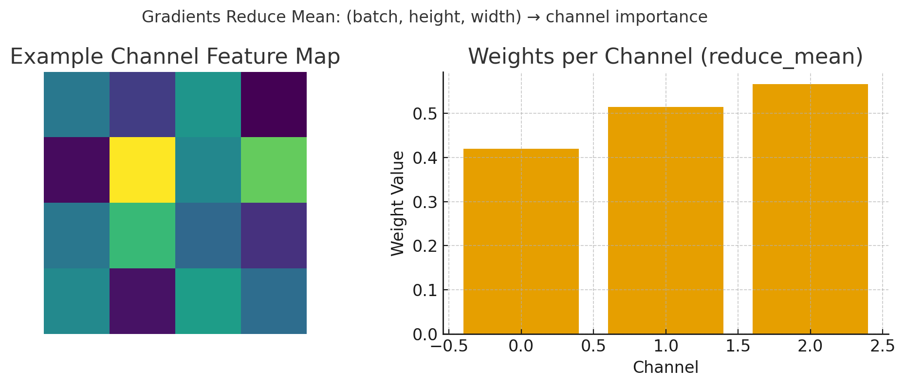
รูป: การคำนวณ Gradient weights - แสดงการ reduce mean จาก feature map (ซ้าย) เพื่อหาค่าความสำคัญของแต่ละ channel (ขวา)
🎨 Step 3: สร้าง Heatmap - แผนที่ความสำคัญ
1. นำ weights (ความสำคัญ) คูณกับ feature maps
2. รวมทุก channel เข้าด้วยกัน
3. ใช้ ReLU (ตัดค่าติดลบออก - เก็บแต่ส่วนที่ส่งผลบวก)
4. ปรับขนาดให้เท่าภาพต้นฉบับ (20×20 → 350×350)
# สร้าง weighted activation map
heatmap = np.sum(weights * last_conv_output, axis=-1)

# ReLU - เก็บแต่ค่าบวก (ส่วนที่สนับสนุนการตัดสินใจ)
heatmap = np.maximum(heatmap, 0)

# Normalize ให้อยู่ในช่วง 0-1
heatmap /= np.max(heatmap)

# Resize กลับเป็นขนาดภาพเดิม
heatmap = cv2.resize(heatmap, (350, 350))
• สีแดง = พื้นที่ที่ AI สนใจมาก (น่าจะเป็นจุดติดเชื้อ)
• สีเหลือง = พื้นที่ที่ AI สนใจปานกลาง
• สีน้ำเงิน/โปร่งใส = พื้นที่ที่ AI ไม่สนใจ
🔬 ทำไม GradCAM ถึงสำคัญในทางการแพทย์
✅ สร้างความเชื่อมั่น
แพทย์เห็นว่า AI มองจุดเดียวกับที่แพทย์สนใจ ไม่ใช่ดูพื้นหลังหรือขอบภาพ
🔍 ตรวจสอบความถูกต้อง
ถ้า AI มองผิดจุด (เช่น ดูที่ตัวอักษร X-ray แทนที่จะดูปอด) แพทย์จะรู้ว่าโมเดลมีปัญหา
📚 เป็นเครื่องมือสอน
นักศึกษาแพทย์เห็นว่าจุดไหนของภาพ X-ray ที่บ่งบอกถึงความผิดปกติ
🛠️ การใช้งาน GradCAM ในโปรเจกต์นี้
ขั้นตอนการใช้ GradCAM กับภาพ X-ray
• โหลดภาพ X-ray ที่ต้องการวิเคราะห์
• เตรียมโมเดล CNN ที่ train แล้ว
• ใช้ last_conv_layer (Conv2D 128 filters)
• Layer นี้มี high-level features
• Forward pass + Backward pass
• สร้าง heatmap ขนาด 20×20
• Resize heatmap เป็น 350×350
• ใช้ colormap 'jet' (น้ำเงิน→เขียว→เหลือง→แดง)
• Overlay heatmap บนภาพต้นฉบับ
• Alpha = 0.5 (ความโปร่งใส 50%)
📊 ตัวอย่างการแปลผล GradCAM
| ลักษณะ Heatmap | การแปลผล | ความน่าเชื่อถือ |
|---|---|---|
| จุดสีแดงอยู่ที่ปอดพอดี | AI มองถูกจุด ตรงกับพยาธิสภาพ | ✅ สูง |
| สีแดงกระจายทั่วปอด | อาจมีการติดเชื้อลุกลาม | ⚠️ ปานกลาง |
| สีแดงอยู่นอกปอด | AI อาจมองผิด หรือมี artifact | ❌ ต่ำ |
| ไม่มีจุดสีแดงเด่นชัด | AI ไม่แน่ใจ หรือภาพปกติ | 🔍 ต้องตรวจเพิ่ม |
⚠️ ข้อควรระวังในการใช้ GradCAM
1. GradCAM ไม่ใช่การวินิจฉัย - เป็นแค่การแสดงว่า AI มองอะไร
2. ต้องมีความรู้ทางการแพทย์ - ในการแปลผล heatmap
3. อาจมี false positives - AI อาจมองเห็น pattern ที่มนุษย์มองไม่เห็น
4. ขึ้นกับคุณภาพโมเดล - ถ้าโมเดลไม่ดี GradCAM ก็จะไม่มีความหมาย
🏥 การนำไปใช้งานจริง
ขั้นตอนการใช้งานระบบ
📝 สรุป
🎯 Key Takeaways
- CNN เหมาะสำหรับการวิเคราะห์ภาพทางการแพทย์ด้วยความแม่นยำสูง
- การ Train Model ต้องจัดการ data imbalance และใช้ augmentation
- การประเมินผล ต้องดูหลายตัวชี้วัด ไม่ใช่แค่ accuracy
- LLM ช่วยให้คำอธิบายที่มนุษย์เข้าใจได้
- การใช้งานจริง ต้องมีแพทย์ตรวจสอบเสมอ
📌 ข้อความสำคัญ: ระบบ AI นี้พัฒนาขึ้นเพื่อเป็นเครื่องมือช่วยแพทย์ในการคัดกรองเบื้องต้น ไม่สามารถใช้แทนการวินิจฉัยโดยแพทย์ผู้เชี่ยวชาญ ผลการวิเคราะห์ต้องผ่านการพิจารณาจากแพทย์เสมอก่อนการรักษา